NtupleTutorial
Introduction
When you want to perform a physics analysis, you need a way to access and manipulate the data. For Mu2e, this could include evaluating the performance of the tracking chamber, calorimeter, or cosmic ray veto detector. You might want to look at "raw" information from the detector, like voltages or waveforms, or you might want higher-level quantities, where hits from the tracking detector have been combined into tracks or energy deposits in the calorimeter have been clustered into total particle energy. Whatever you need to do, you need a way to extract the information that you need.
At its most basic, you can think of an Ntuple as a database. It has variables defined that are filled with information. There are many different formats your Ntuple can take, depending on what information you want to access. In this tutorial we will work with a basic tracking Ntuple. We will learn how to discover what information the Ntuple contains and how to access and display that information. Hopefully what you learn here will translate to other Ntuples that you face in the future.
Note that much of the work we'll do is related to learning how to work with ROOT, a common plotting/fitting program used across many experiments in particle physics. There are many root tutorials out there that you might find useful before, during, or after going through this tutorial.
Setting up your ROOT environment and accessing the Ntuple
Before we begin looking at the Ntuple, please enter into your muse working directory and make sure the Offline environment is set up (mu2einit and then muse setup). There are two Ntuples created for you to explore during this tutorial. They include information from the tracker, but also a ton of other information (fix wording here). One includes signal and background events, while the other just has signal event information. We will focus on the latter.
The files are located at
/cvmfs/mu2e.opensciencegrid.org/DataFiles/tutorials/trkana_signalAndBkg.root
/cvmfs/mu2e.opensciencegrid.org/DataFiles/tutorials/trkana_signal.root
If the files are small, you can copy the ROOT files into your own working directory using the cp command. However, you can also access the tutorials by using the full pathway (/cvmfs/mu2e.opensciencegrid.org/DataFiles/tutorials/trkana_signal.root) in the command line and not just the name of the root file (trkana_signal.root).
Become Familiar with the Ntuple
Ntuple files contain lots of information. It is extremely helpful to know how the Ntuple was made. Without that information, you may not know what units are being used for different variables. (NEED TO FILL THIS OUT MORE...any other ideas? Plus a place to point them towards to learn this info
To open the Ntuple file type: root -l trkana_signal.root (the -l is optional but stops the root logo from popping up when you open ROOT). This opens the ROOT environment and allows you to navigate through the Ntuple. There are two ways to see the structure of the Ntuple: using a TBrowser, which opens an interactive window where you can click through the folders, and using the ROOT command line.
To set the Ntuple as your starting file, type: TFile *f1 = new TFile(" /cvmfs/mu2e.opensciencegrid.org/DataFiles/tutorials//trkana_signal.root");
Then to see the first folder, type: f1->ls();
You should see this on your terminal screen:
TFile**		trkana_signal_forENE.root
 TFile*		trkana_signal_forENE.root
  KEY: TDirectoryFile	TrkAna;1	TrkAna (TrackAnalysis) folder ==
Browse with the TBrowser
Once ROOT is open, type in new TBrowser . Now you can look at the file structure! At the top of the left panel should be the trkana_signal.root file. From there you can click on TrkAna folder and the trkana subfolder (called a Tree). Now you have a list of 12 branches in your tree visible to you!
Here is the general info a few of the branches contain:
evtinfo: event level info
dem: results of downstream e minus fit
uem: results of upstream e minus fit that are coincident with the downstream e minus track
dmm: results of downstream mu minus fit that are coincident with the downstream e minus track
demc: calorimeter info for downstream e minus
demmc: MC info for downstream e minus
demmcgen: MC generator info for downstream e minus (i.e. the particle that was created)
demmcent: MC info for downstream e minus at entrance to tracker
demmcmid: MC info for downstream e minus at middle of tracker
demmcxit: MC info for downstream e minus at exit of tracker
Remember this Ntuple is filled with information from the tracker that follows a particle's path through the detector. Thus it contains information from the fits for downstream and upstream moving electrons in the straw tracker, information from the calorimeter (located behind the straw tracker), and the Monte Carlo (MC) information which can be thought of as our "truth" information. The MC shows us how well our tracking information accurately reconstructs the simulated event data.
Explore a Single Branch
Click on the dem branch. Here you have 34 different leaves! Have you noticed the Tree, Branch, Leaf structure of the Ntuple yet? This cute naming convention makes it easy to understand the hierarchical structure of the Ntuple. These leaves are histograms that contain various information about the downstream electron fit. We will look at just a few of them, but feel free to explore more on your own.
Click on the status leaf. There are 2 peaks, one at 0 and one at -1000. A value of >0 is a success, and you can see that about 333/593 entries were a success! You can move the legend box by clicking and dragging on it. Placing your mouse at the top of the bin at 0 will give you the bin contents on the bottom right hand side of the screen.

The next leaf is the pdg , or particle id number. A pdg value of 11 is an electron, 13 is mu-minus, and -11 is positron. (ADD link to PDG website with all the pdg numbers)
Then we have nhits: the number of hits on the track. If no track is found, we have 0 hits, but the sucecssful tracks range from 15-82 hits.
Then we have the ndof leaf that has the number of degrees of freedom in the fit for the tracker hits.
The nactive leaf shows the number of hits used in the fit. The histogram looks similar to the nhits histogram but is not quite the same. You can see the mean value decreased from 21.88 to 21.44. The ndouble is the number of double hits in the tracker, which is when there are 2 hits in the same panel. The straws are on horizontal panels so two hits could mean a more parallel moving particle or more than one particle. Then ndactive is the combination of nactive and ndouble.
Further down there is the t0 leaf has the time of the track. This is when the track is estimated to have crossed z=0. This position is before the tracker begins in our detector, so it is extrapolated backwards using the fit. Our live window for data taking is between 400 and 1700ns. The next leaf t0err is just the error on the t0 values. We only have a finite resolution in timing with the detector.
The leaf titled chisq is the chi- square value for the fit, which is an indication for how well the fit works for the particle hits. Then the con leaf is the consistency of the chi-square fit.
Working with ROOT in the command line
When we are looking at the plots in the leaves, we are seeing the cumulative data for all events. What if we wanted to just see the information for one specific event? To get this you need to type in the terminal ROOT browser:
root [0] TFile *f1 = new TFile(" /cvmfs/mu2e.opensciencegrid.org/DataFiles/tutorials/trkana_signal.root");  (to establish the Ntuple as your starting point)
root [1] TTree *t = (TTree*)f1->Get("TrkAna/trkana");   (to get the trkana tree from the TrkAna folder in the ntuple)
root [2] t->Show(10)   (to get the information for event 10)
Now you should see a lot of information printed out that starts with:
eventid         = 13
runid           = 4001
subrunid        = 0
evtwt           = 1
beamwt          = 1.32845
genwt           = 1.32845
nprotons        = 51809437
nsh             = 1531
nesel           = 1929
nrsel           = 2416
...
The first 3 pieces of information are from the Art Header. The eventid is the art event number. This can have various definitions depending on the sample you are looking at. For pure signal, it represents one conversion electron, but in a mixed signal and bkg sample, it represents one microbunch. The runid is the run number and subrunid is the subrun number.
Next comes the event level information. evtwt is the weight of event calculated by taking the beam weight * gen weight. The beam weight is the weight contribtuion from the proton bunch intensity. In Mu2e this is calculated as number of protons proton/3.9e7. 3.937 is the number of POT (Proton on Target) per microbunch, so this is the mean value of protons expected to hit the production target. The number will change cycle to cycle based on the beam dump intensity, but not from microbunch to microbunch during a cycle from a single beam dump. genwt is the weight contribution from generated particle. This number is assuming that there is only one conversion electron in each microbunch. nprotons is the number of protons assumed for this microbunch.
The next numbers are tracker information. nsh is the total number of straw hits in the event. This is also the number of hits in the tracker. nesel is the number of straws that pass the preliminary energy selection. Protons that are unwanted for our signal tend to deposit much higher amounts of energy than a conversion electron. nrsel is the number of straw hits that pass the radial selection. This removes hits that are close to the inner or outer edge of the tracker. ntsel is the number of straw hits that pass the time selection such that the hits are during a set time window when we expect the conversion electron to interact with the tracker. nbkg is the number of "classified" background straw hits, nster is the number of straw hits with stereo information (when a particle hits 2 separate straws that are close together), and ntdiv is the number of straw hits with time division information (using the signal propagated to both ends of the straw to determine the position on the straw where the particle hit).
Further down there is Track Count Information. ndem is the number of downstream electron tracks, nuem is number of upstream electron tracks, and ndmm is the number of downstream mu minus tracks. ndemc is the number of calorimeter clusters matched to the best dem track. After particles travel through the tracker they hit and then deposit energy into the calorimeter. Based on the track's helical shape, we can predict where on the calorimeter the particle should hit. If there is then a calorimeter cluster at or near that place, it further supports the track being a conversion electron signal. ndemo is the number of shared hits between the primary and next best track found by the tracking algorithms. We try many fits for potential tracks by choosing different starting points, angles, etc. and thus some tracker hits may belong to more than one track fit. ndmmo is the number of hits between the primary and muon-fit track.
There is also calorimeter information and MC information printed out, but we will not go into detail for those leaves here. You are welcome to explore the header files that helped fill those histograms (TrkDiag/ing/TrkCaloInfo.hh and TrkDiag/inc/TrkInfo.hh).
Build a simple analysis structure
Another way to interact with the Ntuple is by creating a Make Class Analysis loop. This creates a .C file and the corresponding .h header file. This allows you to make plots of the variables in a ROOT macro. It also shows you all the information included in the Ntuple in the header file.
Try running these commands:
root [0] TFile *f1 = new TFile("/cvmfs/mu2e.opensciencegrid.org/DataFiles/tutorials/trkana_signal.root");
root [1] TTree *t = (TTree*)f1->Get("TrkAna/trkana");
root [2] t->MakeClass("TreeAnalysis");
Info in <TTreePlayer::MakeClass>: Files: TreeAnalysis.h and TreeAnalysis.C generated from TTree: trkana
[0] is to establish that you are using the Ntuple)
[1] Gets the tree TrkAna from the Ntuple
[2] Makes the macros, the words in "" are the name of the macros you create
You can then browse the .C and .h files using your favorite editor (emacs, vim, etc.)
In the TreeAnalysis.C file you will see that it includes the TreeAnalysis.h file and some basic ROOT macros. Then the Tree Analysis loop starts. You put the code in here that you want the macro to run. The commented section in red gives you some more commands you can run in ROOT. I will explain how to add code to the macro below in the Making Plots section.
Now that you know how to browse the Ntuple, let's start making plots!
Making plots
There are two main ways to make plots: interactively using the ROOT terminal and in the macro you created above (TreeAnalysis.C)
Interactively
You can create a separate canvas and plot any of the histograms included in the leaves of the ntuple. You just need to know the name of the leaf you want to plot. Follow these steps:
root [5] TCanvas *myCanvas = new TCanvas()
root [6] t->Draw("nhits")
[5] create a canvas to have your histogram drawn on
[6] here nhits is the leaf you are plotting

If you have the TBrowser open, your chosen plot will show up there and not in the canvas.
What if you only want to look at a subrange of the data on the histogram? You can change the range by specifying the value in the Draw command.
root [7] t->Draw("nhits", "nhits>15");

Now we can better see the distribution to the left of 15. A more stark example is looking at the momentum leaf. Compare the distributions for momentum of track that you see in the two different histograms created below:
root [8] t->Draw("mom");   ---  unmodified histogram with peaks at -1000 and 100
root [9] t->Draw("mom", "mom>50");  ---  you can actually see the momentum distributions for the downstream electrons' tracks.
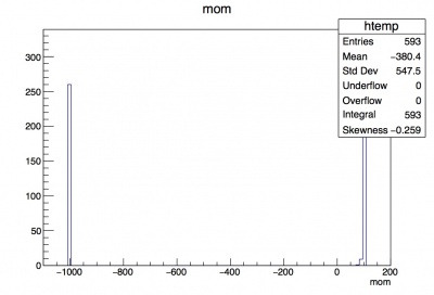
Momentum plot without any cuts
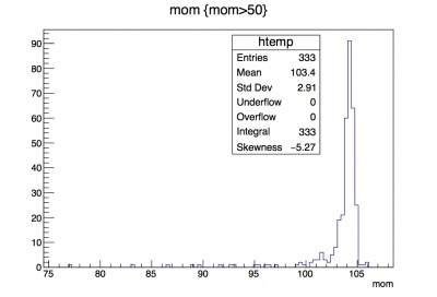
Momentum plot with the cut >50 MeV


With a macro
Back to the TreeAnalysis.C macro we created earlier. To create a single histogram, you first need to book it near the start of the histogram, then fill it with the event information for each hit (in the for loop), and then draw the histogram. We will make a histogram of the number of track hits. The histogram will appear in the TBrowser (so make sure one is still open before you run the macro).
if (fChain == 0) return; | black}}
--- Need to book the histogram here To declare the histogram use this command:
TH1* ndofhistdem = new TH1D ("ndofdem", "Histogram of NDOF for dem", 100, 0, 100);
where TH1* says it will be a 1-dim histogram and ndofhistdem is the name you will use to refer to the histogram in the script. The first command in the paranthesis is the short hand name that will be in the plot legend, the second phrase is the title of the histogram, and then the number of bins, xmin, xmax.
Long64_t nentries = fChain->GetEntriesFast();
Long64_t nbytes = 0, nb = 0;
for (Long64_t jentry=0; jentry<nentries;jentry++) {
Long64_t ientry = LoadTree(jentry);
if (ientry < 0) break;
nb = fChain->GetEntry(jentry); nbytes += nb;
// if (Cut(ientry) < 0) continue;
--- In the for loop portion of the code you need to fill the histogram
ndofhistdem->Fill(dem__ndof)    ---- you need to specify both the branch and leaf value you want to fill
}
the drawing of the histogram goes here:
ndofhistdem->Draw();
}
Now to run and create your histogram, you need to open up ROOT. Then you need to load the code :
.L TreeAnalysis.C
then you need to create an object (a) for the macro:
TreeAnalysis a
lastly you run the loop over the ntuple:
a.Loop()
Drawing 2 Histograms on Same Canvas
What if you want to compare the distribution of one variable for two different track types? You can stack the histgrams on top of each other and compare their distributions. We are going to compare the number of hits in the track for downstream e minus fit and the downstream mu minus fit. Using the same TreeAnalysis.C macro, add a second histogram in the same way as the first, but naming it ndofhistdmm and changing the corresponding dem -> dmm changes. To make the distributions easier to differentiate, change the color of the second histogram by
ndofhistdmm->SetLineColor(kMagenta): (you can also use kGreen, kRed, kYellow, etc.)
Then the one difference is that you need to add Draw("same") after you draw the first histogram.
ndofhistdem->Draw();
ndofhistdmm->Draw("same");
You can see that the two types of fits have very similar distributions, but this may not always be the case. Stacked histograms can help us choose where to make selection cuts in our trigger and analysis in order to separate signal from background!

Making a 2D histogram
You might also want to see if there is a correlation between two different variables. For example, the number of hits used in the downstream electron fit (nactive) and the number of double hits used in the same fit (ndactive). This is similar to plotting the single variable on the histogram except you change the TH1* line to:
TH2* hits2D = new TH2D ("hits2D", "Histogram of nactive vs. ndactive hits", 100, 0, 100, 100, 0, 100);
where you have defined it a 2D histogram (TH2*) and have at the end of the paranthesis bins1, xmin1, xmax1, bins2, xmin2, xmax2
Then when you fill the histogram you have to fill both variables:
hits2D->Fill(dem__nactive, dem__ndouble); where you fill (xval, yval)
The plot should then look like this (after you compile and run the macro):

If you want it to be in color then go to the browser and click on View -> Editor . Then click on the physical data points on the plot. Then tick the boxes for Col and then Palette (your legend). You might need to move the legend to fully see the color palette. The plot should now look like this:

The End
Hopefully, you feel like you can work your way around a ROOT file by using the browser and creating an analysis macro. There is so much more that can be done in ROOT. Feel free to work through a few other tutorials that can be found on the web. Almost any technical problem, such as how to not show the legend for the second histogram when you stack them ( gStyle->SetOptTitle(0);), can be found by googling.
This tutorial features one instance of a kind of ntuple, called TrkAna, but there are other choices. You can make a new TrkAna ntuple for an art file you have, or you could make other kinds of ntuples with other formats and other contents. For example, you can create an ntuple that contains only the information you need for a particular project or goal. Or you could modify the contents of an existing ntuple. In making these decisions, probably the most important factor is the ability to share datasets, tools and expertise with the people you will be working with, so you should consult with your mentor and group leader.
If you have complete freedom, or want to explore what is possible, you can take a look at the Ntuples page.
Good luck!